Monte Carlo Simulation for Startup Valuation
How to assess valuation uncertainty when future outcomes depend on many uncertain variables.


So far, we have discussed the valuation of innovative ideas by constructing scenarios based on expected inputs and outcomes. We distinguished between pre-money valuation, post-money valuation, and a future or opportunistic value that reflects the potential upside of a startup. While this approach is useful, it raises an important question: how reliable is a valuation that depends on many assumptions about an uncertain future?
The question now arises: how reliable is this valuation? The pre-money and post-money valuations are generally straightforward, i.e., the costs incurred so far to create the product, representing the pre-money valuation, and the pre-money valuation plus the investment, representing the post-money valuation, which we know may include some goodwill or badwill.
It's different for the opportunistic value that might be achieved. Here, many factors play a role that are often difficult to predict accurately. Yet, there is a tendency to present the proposed scenario and the derived opportunistic value as the truth. Of course, this is not the case, but what can be done about it? One option is to use your spreadsheet to perform a sensitivity analysis, by varying the number of iCics sold, for example, and then observing the effect on EBITDA. Or you could vary the costs to see the impact—whatever you choose. This way, you could explore where your break-even point lies, i.e., the minimum number of iCics that must be sold to avoid going into the red. A break-even analysis is certainly recommended to test the robustness of the scenario reflected in the budget.
It becomes more challenging when you want to test multiple variables simultaneously, especially when you need to investigate the effect of one variable on another, particularly if the relationship is non-linear. In the case of the iCic, this should be manageable. We can simply play with the 'input variables' and see how rich (or poor) we will become if more (or fewer) than a certain number of iCics are sold in the future. Of course, we should not forget that if sales decrease, production will also slow down, reducing variable costs. This is still manageable and should not be a problem for most innovations. However, in other cases, problems may arise that we need to be prepared for.
Let's return to our startpage with "The Three Pillars of an Invention". There, I already warned you about the risk that the invention may be rejected due to safety concerns. In the case of the iCic, for example, there is uncertainty about whether it will be allowed to be used in the car while driving (we already know it likely won't be, but this is just an example); perhaps the iCic may only be used while parking, or there is even a chance that the iCic will not be allowed to be installed by the government at all. If the latter occurs, it does not necessarily mean that there are no applications for the technology, but the scenario would change significantly.
In the paragraph above, there are four important words: risk, uncertainty, probability, and change; you can already sense where this is headed—we are now entering the realm of statistics. Now, I would be the first to admit that it's completely 'over the top' to apply statistics to the iCic or your invention at this stage. In fact, make sure your invention works first and that you have a solid business plan to present to your future investor and/or partner. However, this could be different if your invention is something in the life sciences, which is a very different field. The method/technique I will briefly cover below is applicable in many areas, but is typically used when very large investments need to be made and there is significant uncertainty regarding, for example, the R&D trajectory or regulations, just to name a few. To manage this uncertainty, Real Options and Monte Carlo Simulation (MCS) are often used. Here, we will only cover the MCS.
Sensitivity Analysis
During a sensitivity analysis, one or more key variables (e.g., revenue, market share, costs, whether or not government approval is granted to launch the product, etc.) are varied to observe the effect on the NPV. In other words, we study the consequences if an (important) estimated variable takes on a different value than originally projected in the DCF model. For example, in the page with the comparables table, we assumed a revenue value of 110 million for simplicity. We never explained how we arrived at this figure, as it was not relevant to the discussion at the time, but let's assume we considered this value most likely because we expect 100,000 iCics to be sold at a price of 1,000 euros each. With a simple sensitivity analysis, we can now see the impact on the 'bottom line' if, instead of 100,000, only 75,000 or 50,000 are sold; or, of course, what happens if 200,000 units are sold instead of 100,000. Similarly, we can vary the price or any other variable.
Monte Carlo Simulation for Startup Valuation
During an MCS analysis, however, the probability that a variable will take on a certain value is examined. For this, a distribution with a mean (μ) and standard deviation (δ) is assigned to the variable in question. In the case of revenue in the above example, we could, for instance, assign a normal distribution to the number of iCics sold, with a mean of 100,000 and a standard deviation of 15,000. This is represented as N(μ,δ), where N stands for the normal distribution with μ = 100,000 and δ = 15,000.
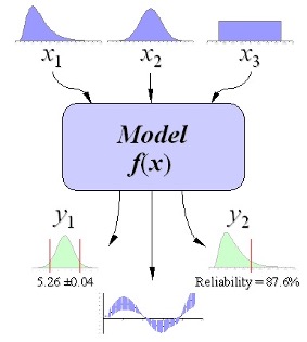
Monte Carlo simulation is then the procedure where many possible scenarios are run in a decision support system in a fast, automated way to obtain an estimate of the uncertainty associated with the modeling. We saw earlier that the assigned value of each input variable and/or key driver is actually a mean, or expected value (best guess estimate), and even if the variance around the expected value of the variable is known, it is not taken into account in determining the value. Monte Carlo simulation provides a solution to this. Monte Carlo simulation makes it possible to incorporate the variance, or risk, by assigning a distribution to the input variables with a corresponding mean (μ) and standard deviation (δ). At each draw, a value is assigned to the variable according to the specified distribution. This drawn value is used in a model to calculate the NPV. All the calculated NPVs themselves also form a distribution with their own μ and δ, providing a comprehensive insight into, among other things, the volatility.
While uncertainty in future cash flows can be explored using sensitivity analysis or Monte Carlo simulation, the question remains how investors translate risk into a required return. In practice, this is often done by adjusting the discount rate rather than the cash flows themselves. One widely used framework for this is the Capital Asset Pricing Model (CAPM) , which links risk to expected return through market exposure and systematic uncertainty.
Monte Carlo simulation does not replace traditional valuation methods such as DCF or comparables; instead, it complements them by explicitly showing how uncertainty affects valuation outcomes. Rather than producing a single point estimate, it reveals a distribution of possible values and makes clear how sensitive a startup's valuation is to assumptions about market adoption, pricing, costs, and risk. For investors, this probabilistic view is often more informative than a single number, as it connects expected returns, downside risk, and the assumptions embedded in the discount rate. In that sense, Monte Carlo simulation represents the final step in our valuation series: moving from deterministic models to a realistic, risk-aware understanding of what a startup might truly be worth.
Monte Carlo simulation is a powerful tool for modeling risk under uncertainty, but it fundamentally assumes that uncertainty can be expressed as probability distributions. In some innovation-driven cases, this assumption breaks down entirely. When future value depends on technological breakthroughs that create new markets or platforms, the uncertainty is not probabilistic but fundamental. Such outcomes do not reside in the tail of a distribution — they exist outside the distribution altogether. A clear example is the development of mRNA technology by Moderna , where value creation could not be meaningfully modeled using probabilistic methods. Monte Carlo simulation models risk, not fundamental uncertainty — truly transformative innovations do not sit in the tail of a distribution but outside the distribution altogether.